Probability distributions:
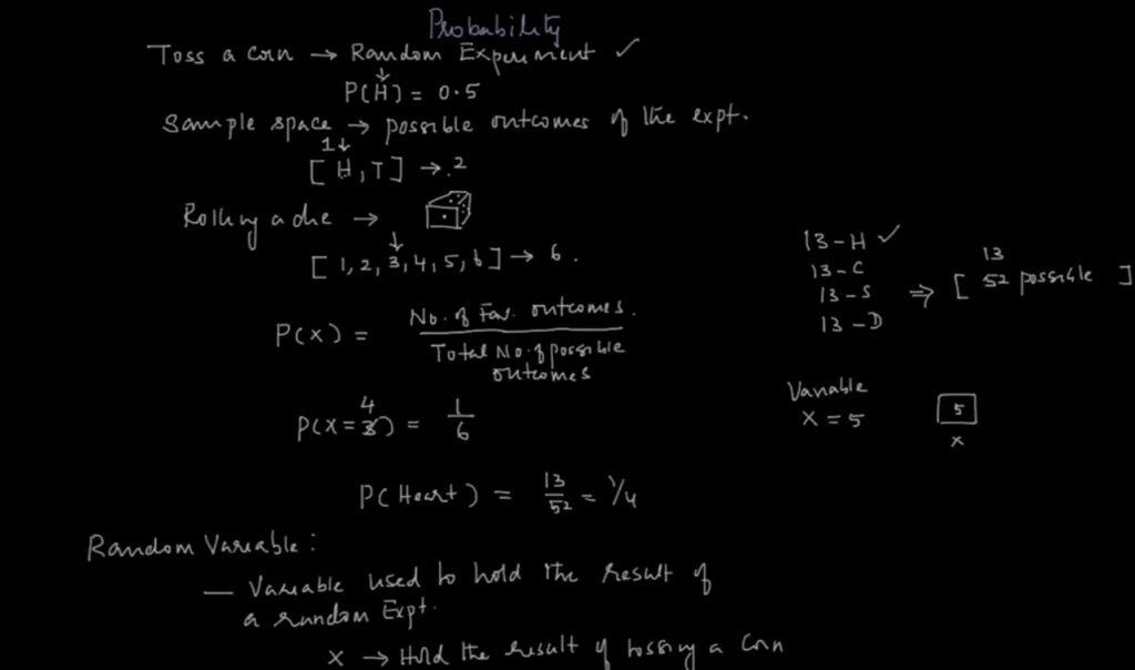
Case: People who don’t smoke live longer than people who smoke. random variable: Any variable which is subjected to chance and the behavior of random variable is governed by their probability distributions.
On studying a small group of people who smoke daily and then compare them with another small group of people who don’t smoke. This is called sampling.
For each of these 2 small groups, we will try and form a Hypothesis what might be true for all people and see if this Hypothesis is supported or not supported by statistics.
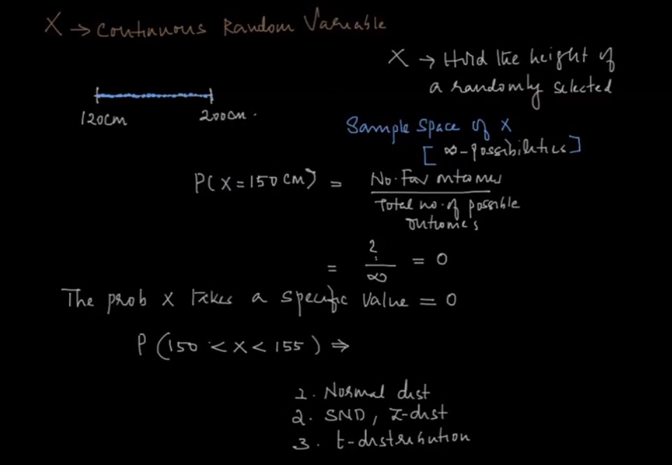
Continuous Random variables:
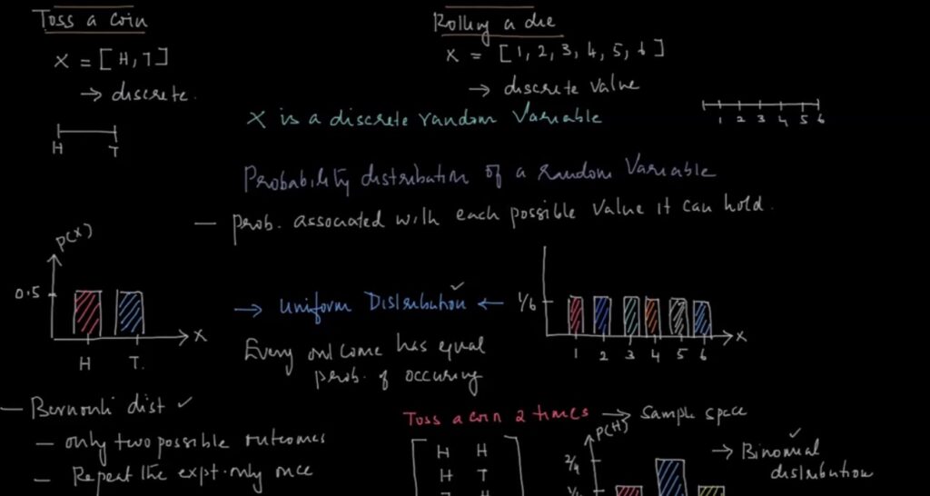
Random variables are variable
– Whose value cannot be determined before an event happens.
– Whose value is subject to variation due to chance, but we know the value is restricted to a finite set of values.
Now let’s take a problem like fraud detection. To detect any fraudulent card transaction, we need to identify those variables which are related to a card transaction and can influence the problem. Below are few such variables and their types.
1. Amount spent (0 to ∞) – Continuous
2. IP address (set of all IP address in the world) – Categorical
3. Number of failed attempts on using the card (0, 1, 2.. ) – Discrete
4. Time since last transactions (0 … ∞) – Continuous
5. Location of transaction (Austin, Dallas, New York) – Categorical
As we see, each of these variables can have some influence on the transaction. We will not know the value of these variables before the transaction occur but will know the range for their values. And for each transaction, each variable’s value will be different, but it has to be from with in this set of range.
Statistical Experiment :
Tossing a Die:
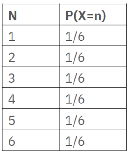
statistical experiment is tossing a die. When we toss a die, we will not know which value will come up, but we will know it has to be one of the values from 1 to 6. The outcome of a statistical experiment is represented by random variable.
In this case let say the outcome of the toss is X. Now X will be a discrete variable as it can take value from 1 to 6 all integers. Below table links each possible value of X with its probability.
LinkedIn user’s group:
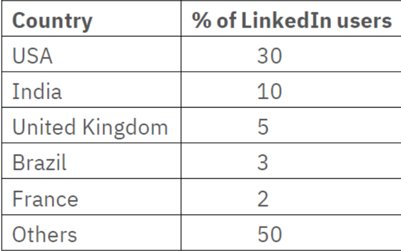
Below statistic report showing LinkedIn user’s top 10 geographical distribution. Let say we need to pick a user at random from the entire group of LinkedIn user, and tell what country they are likely to be from. In a statistical experiment – whose set of outcomes can be specified beforehand, but the actual outcome of the experiment is subject to chance.
Please note here the country of the user will be random variable which usually will be represented as X. Probability distribution is a table or function that links each outcome of a statistical experiment with its probability of occurrence.
P (the person picked is from USA) = P(X) = 0.3 (from above table)
Normal distribution:
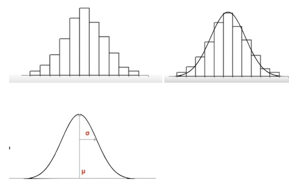
In normal distribution, most of the measurement (say height of a person) will be concentrated in the central peak. And there will be very few measurements that are very far off from the central point. Now these measurements are drawn from probability distribution which is basically a normal distribution. – X axis is the value of the random variable.
– Y axis is the probability that it can take.
– The peak is the mean or the average value.
– Most of the measurement will be concentrated around the mean or average value.
– The spread of the distributions is described by the standard deviation.
– In other word, given the mean and SD, we can tell the probability of any value.
Empirical Rule:
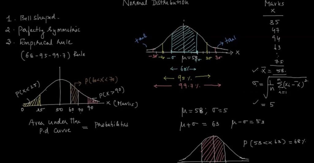
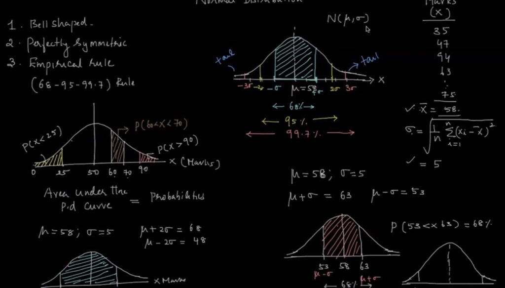
If we know the mean, SD you can tell the probability of any value that can occur in the normal distribution.
– Regardless of the actual values of mean and SD some characteristic remains same.
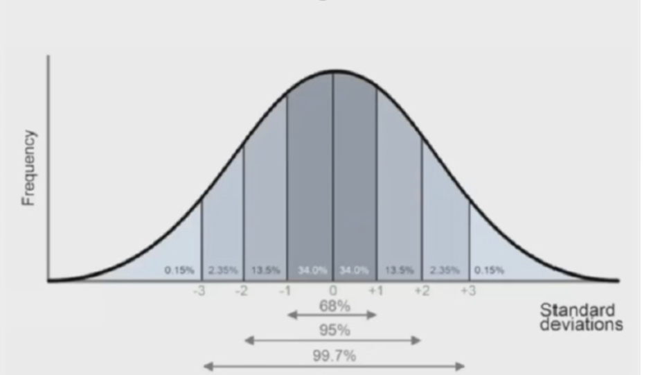
– Probability that a value lies within 1 SD either direction from the mean is always 68%
– Probability that a value lies within 2 SD in either direction from the mean is always 95%
– Probability that a value lies within 3 SD in either direction from the mean is always 99.7% Above rule is very useful for
1. Testing whether a distribution is NORMAL
2. Finding outliers: Any values more than 3 σ away from the mean can be treated as outliers
Sampling:
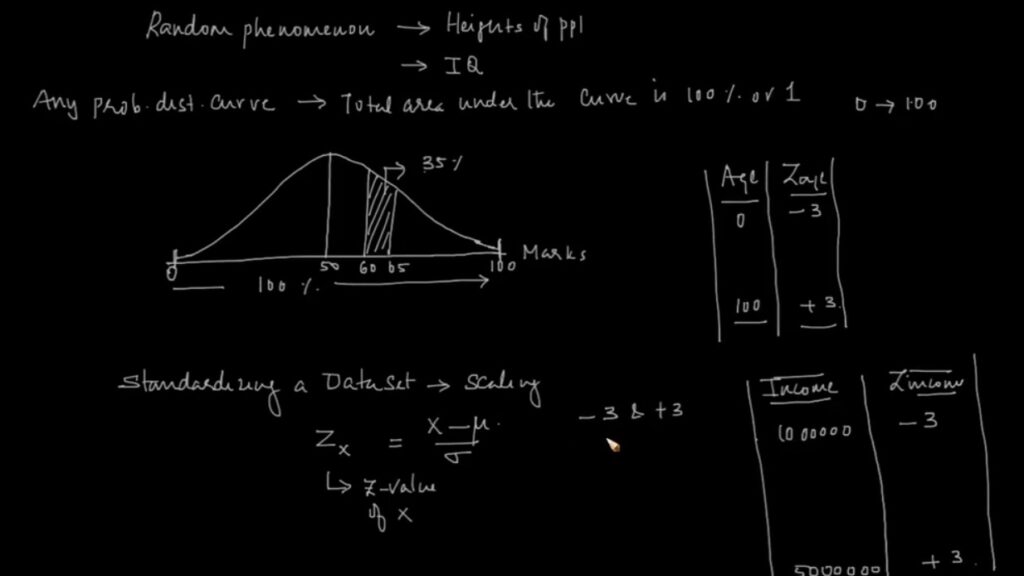
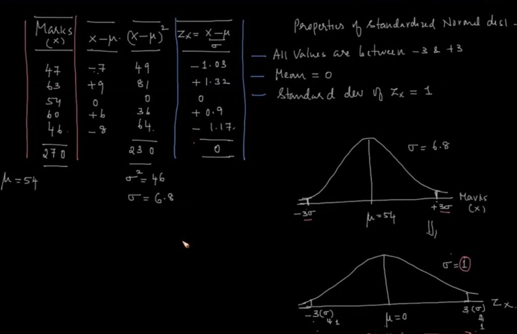
Standardizing a dataset:
In simple word, Sampling means drawing conclusions about the population by observing the sample and generalizing. The conclusion which we draw is called inference. To draw meaning inference, we learn few techniques and hypothesis testing.
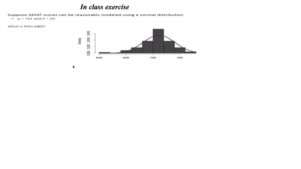
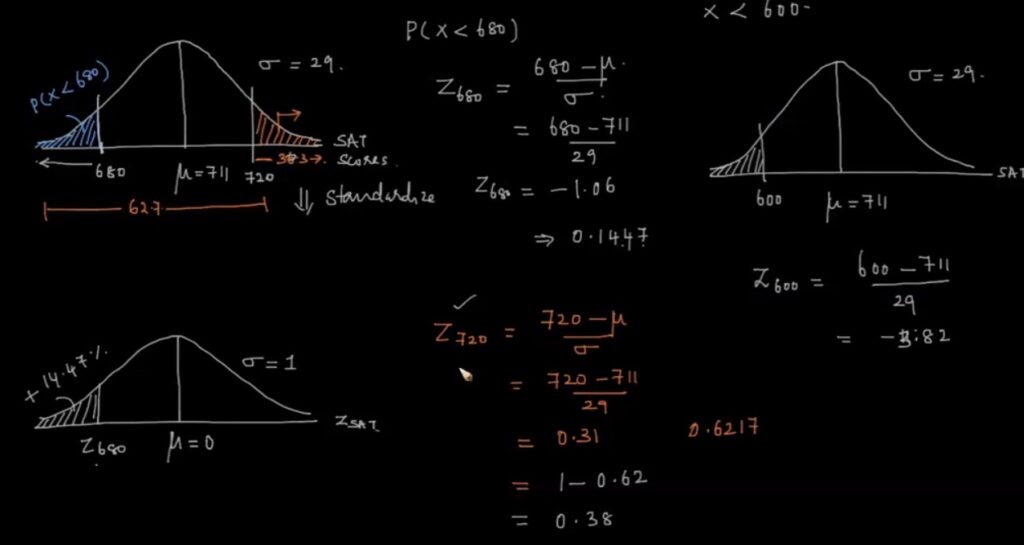
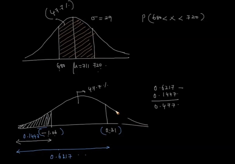
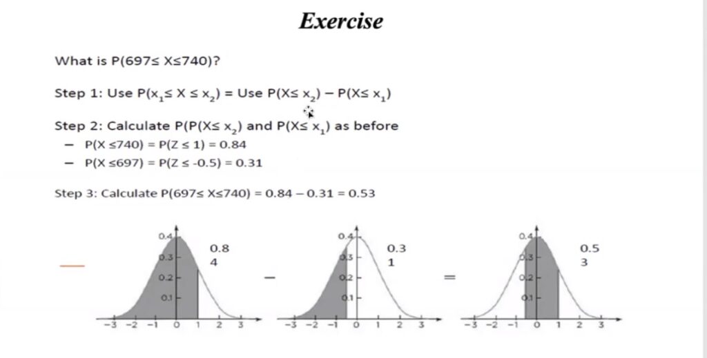
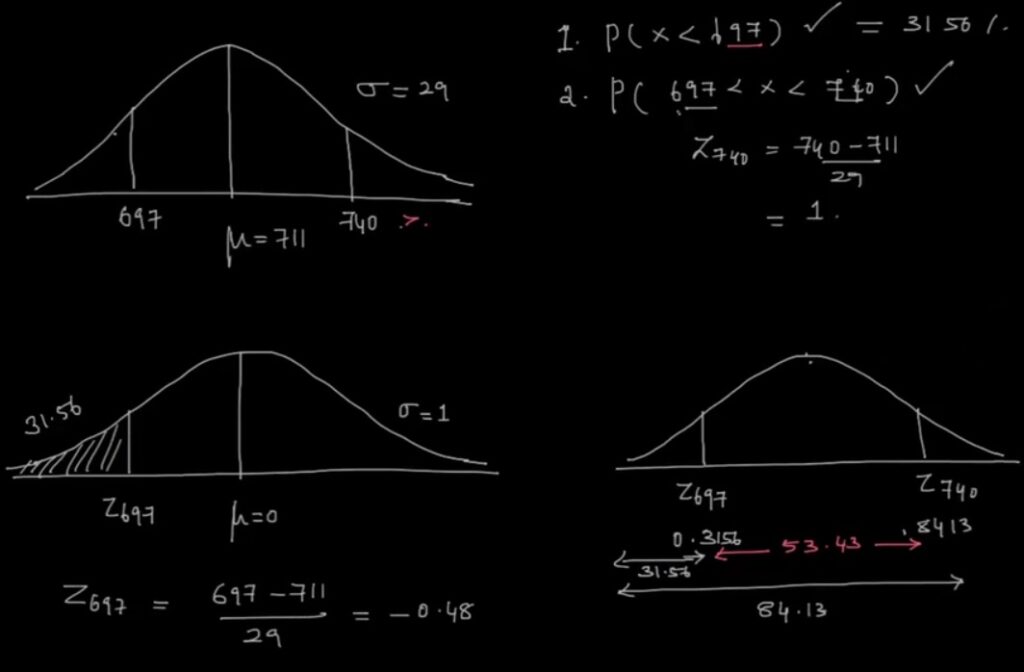
Practice problem probability of normal distribution:
Recent Comments